The Fast Fourier Transform (FFT): Most Ingenious Algorithm Ever?
May 30, 2021The world of
algorithm
s is vast, but we can often divide them into two distinct classes. The first class are those that are intrinsically useful. Think of your standard graphalgorithm
s like dfs or bfs. These algorithms appearever
ywhere, they are efficient and, as a result. we like to understand them the second class of algorithms we study are those that are simply beautiful, think about the first time you saw the incredibly simple recursive implementation of towers of annoyance, if you have a soul, you feel a sense of wonder, a sense of wonder. Given the elegance of such an algorithm, it turns out that it is actually not that useful or efficient, but we still study it in the same way that we like to read a work of fiction, it inspires us and motivates innovative thinking. today I want to talk about an algorithm that legitimately belongs to both classes and my personal favorite algorithm, thefast
Fouriertransform
, thefast
Fouriertransform
or fft is, without exaggeration, one of themost
important algorithms created in the last century, much of it of the modern technology that we have today, such as GPS wireless communication and, in fact,ever
ything related to the vast field of signal processing is based on the knowledge of FFT, but it is also one of themost
beautiful albums that you have ever seen for the depth and sheer amount of brilliant ideas that I looked at is simply amazing, it is easy to overlook the beauty aspect of FFT as it is often introduced into quite complex environments that require a lot of prior knowledge such as the discrete Fourier transform, time domain to frequency domain conversions and much more, and to be fair.
To get a full appreciation of FFT applications, you can't really avoid any of these ideas, but I want to do something a little different. We will take a discovery-based approach to learning about FFT in a context where you all are. I am familiar with multiplying polynomials, as I see the structure of this video. It's about starting with some common ground and then slowly asking questions that will hopefully lead you to discover the truly
ingenious
ideas behind the fast Fourier transform. Alright, let's start with the configuration here. It's simple, we are given two polynomials and we want to find the product, our task will be to design an efficient algorithm for this problem mathematically we know an algorithm to multiply polynomials by repeatedly applying the distributive property, all of you may have been applying this algorithm instinctively from any algebra class Before trying this idea, although the first question we have to address is the representation of polynomials on a computer, the most natural way to represent them is through coefficients where we assign coefficients to lists, this helps to organize our coefficients in the following order . mainly because now the coefficient of the index k is assigned to the coefficient of the term of degree k, we will refer to this representation as the representation of coefficients of polynomials in general, given second degree polynomials, the product will have a degree of 2 times d and the execution The time of this algorithm, if we actually implement it with the more natural distributive property approach, will be or d squared, since each term of the polynomial a will have to be multiplied by all the terms of the polynomial b.
More Interesting Facts About,
the fast fourier transform fft most ingenious algorithm ever...
The question now is: can we do better? The first really clever idea comes from thinking about polynomials a little differently to see the key idea here, let's look at one of the simplest polynomials, a polynomial of degree one or a linear function, we can represent any line with exactly two coefficients, one for the degree. term zero and one for the term of degree one the key part that makes this representation valid is that each representation has a one-to-one mapping to a single line. What other representations of a line have this property? There are actually several reasonable representations, but the one we're going to use is the two-point representation.

We know from geometry that any line can be represented by two distinct points, and it turns out that there is a clear extension of this to general polynomials, which I will denote here as any polynomial of degree. d can be uniquely represented by d plus a point, for example, if I give you three random points, this means that there is exactly one quadratic function that goes through the three points. If I give you four points, there is exactly one cubic function that happens. Across all these points, this claim is perhaps a little surprising, so it deserves proof.

Suppose I give d plus a single point polynomial of degree d p of x. We want to show that for this set of points there is only one set of coefficients, so if we actually evaluate our polynomial at each of these points and obtain the following set of systems of equations. Whenever you have a system of equations, writing it as a matrix vector product is almost always useful for analysis. A nice property of this matrix is that if each of our original points are unique, as they are in this case, the matrix will always be invertible.
The easiest way to prove this is by calculating the determinant which you will find is not zero, but I will link a good linear algebraic proof of this fact in the description as well, for those interested anyway, what this means is that for For each set of points there exists a unique set of coefficients and, consequently, a unique polynomial. Taking a step back, what this means is that there are actually two ways to represent polynomials of degree d, the first being the coefficient representation and the second with just d plus a point, which we'll call the value representation.
A nice property of using the value representation is that multiplying polynomials is much easier. Let's say I ask you to multiply these two polynomials by x. and b of x we know that the resulting polynomial c of x will be of degree four, so we will need five points to uniquely represent the product. What we can now do is take five points from each of the two polynomials and then simply multiply the function. values one by one to obtain the representation of the value of the product of the two polynomials following our previous rule, there is only one polynomial of degree 4 that passes through these points; that polynomial happens to be next in the coefficient representation and this is in fact the product of our original polynomials a of x and b of x with the multiplication operation performed using the value representation, we have now reduced the multiplication time of our operations d original squared to the order of only operations of degree d, okay, so let's propose a plan to To improve the multiplication of polynomials, we are given two polynomials in the representation of coefficients of degree d, each of which we know that the multiplication is faster using the value representation, so what we'll do is evaluate each of these polynomials in 2d plus 1 point, multiply each of these points in pairs to get the value representation of the product polynomial, and finally, somehow , convert the value representation back to the final coefficient representation.
This is the big plan, but there are several pieces of the puzzle that we haven't discovered. What we're really missing is some type. of magic box that could take polynomials in the coefficient representation and convert them to the value representation and then vice versa, that magic box, my friends and believe me, it is truly magic is the fast Fourier transform, let's focus first on taking polynomials from the representation of coefficients to the representation of the value that we will call evaluation we have a polynomial of degree d and we want to evaluate the polynomial at n points where n is a number greater than d plus one.
Let's think about the simplest way to do this. We can choose random n. coordinates and simply calculate the respective y coordinate, this works, but when we deconstruct what is actually happening here, we run into our old enemy, each evaluation will take d operations, which makes this method run in o of n times d time , which ends up being or d squared to evaluate all the endpoints, so let's go back to where we started, can we find a way to optimize this? Let's try to simplify the problem, say that instead of considering a general polynomial, we wanted to simply evaluate a simple polynomial as p of x is equal to x squared at eight points, the question now is which points should we choose.
Is there any set of points when knowing the value of one point immediately implies the value of another? In fact, if we choose the point x is equal to one, we immediately know the value of the point x is equal to minus one. Similarly, if we choose x is equal to two, we automatically know that value, expanding on this idea, the key property we want here is that our eight points must be positive negative evens, the reason this works is because of the property of even functions where a function evaluated at negative x is going to be equal to the function evaluated at positive x, fine, but then the next immediate question is what about functions like x cubed?
It does the same trick that it actually does, but with one Warning: each positive x value will have the same value as the negative x value, but with the sign reversed, so in these two cases of single-term polynomials of Even and odd degree, instead of evaluating eight individual points, we can get away with evaluating exactly four positive points. from which we immediately know the value of the respective negative points, let's see if we can extend this idea to a more general polynomial, inspired by our initial exploration, let's divide our polynomial in terms of even and odd degrees if we factor out an x of the odd degree. terms we end up having two new polynomials where these new polynomials only have terms of even degree, in fact let's give these polynomials formal names, the first represents the even terms and the second represents the odd terms after factoring x.
This fact allows us to recycle a large number of calculations. between pairs of positive and negative points, an additional fact is that since these even and odd polynomials are functions of x squared, they are polynomials of degree two, which is a much simpler problem than our original polynomial of degree five, generalizing these observations if we have an n minus a polynomial of degree that we want to evaluate at n points, we can divide the polynomial into even and odd terms with these two smaller polynomials that now have degree n over two minus one, so how do we evaluate these polynomials with half the degree of our original polynomial?
The nice thing here is that this is just another evaluation problem, but this time we need to evaluate the polynomials in each of our original inputs squared and this works great since our original points were positive negative pairs, so if we originally had n points now we just end up having n over two points this is starting to smell like the beginning of a recursive algorithm let's look at the bigger picture we want to evaluate a polynomial p of x at the end points where the end points are positive negative pairs we divide the polynomial in components of even and odd degree where we now have two simpler polynomials of degree n over two minus one that only need n over two points to evaluate once we recursively evaluate these smaller polynomials we can go through each point in our original set of end points and calculate the respective values using the relationship between the positive and negative even points, this gives us the representation of the value of our original polynomial.
If we can make this work, this means we have a recursive or n log n algorithm since the two recursive subproblems are half the size of the original problem and take linear time to evaluate the endpoints. This would be a huge improvement over our previous quadratic runtime, but there is a major problem. Can you detect the problem? The problem occurs in the recursive step on which the entire scheme is based. the fact that the polynomial will have even positive and negative points for evaluation, this works at the top level, but at the next level we are evaluating n over two points where each point is a squared value, they all end up being positive, so that recursion breaks, then The natural question is: can we make this new set of points have positive and negative pairs?
Some of you may have already seen it, but this actually leads to the third absolutely
ingenious
idea behind the fft. The only way this is possible is if we expand the domain of possible starting points. to include complex numbers for a special choice of complex numbers, the recursive relation works perfectly where each subsequent set of points will contain positive negative pairs. What possible set of initial endpoints does this property have? This is a difficult question and to answer it we are going to do a little reverse engineering with an example, let's say we have a polynomial of degree 3 that requires at least n equals 4 points for its value representation.These points must be positive negative pairs so we can write them as x1, negative x1, x2, and negative x2.We know that the recursive step will require us to evaluate the even and odd divisions of the polynomial at two points x1 squared and x2 squared. Now the key constraint here is that for recursion to work these two points also have to be positive negative pairs, so we have an equivalence between x2 squared and negative x1 squared at the bottom level of the recursion will have a single point x1 raised to the power of 4. Now the good thing is that we can choose these points, let's see what happens if we choose our initial x1. be 1. This means that two of our starting points are 1 and negative 1, which at the next level of recursion means that x1 squared and negative x1 squared also have to be 1 and negative 1 respectively and at the bottom layer we have just one point that ends up being 1.
Now the question is which x2 should we choose so that when we square x2 we end up with negative 1. The answer is the complex number i, which means that the four points we need to evaluate this polynomial in r 1 negative 1 i and negative i An alternative perspective to what we just did here is that we essentially solved the equation x to the power of 4 equals 1. since in the lower layer of recursion the value of any of our original values points to the power of four was one we know that this equation has four solutions, all of which are encompassed by a special set of points called fourth roots of unity, let's see if this generalizes if given a polynomial of degree 5 we will need n to be greater than or equal to 6 points Since our cursive method divides each problem in half, it is convenient to simply choose a power of two, so let's choose n equals eight.
Now what we have to do is find eight points that are positive negative pairs so that each of these points when raised to the eighth power is equal to one we see that the correct points are the eighth roots of unity generalizing this to any polynomial of degree d, what we will do is choose n is greater than or equal to d plus one points such that n is the power of two and the points that we must choose are the nth roots of unity, this fact deserves a little more explanation why does this work before answering that question, let's formalize a few things, the nth roots of unity are the solution to the following equation and are best visualized as equidistant points on the unit circle the angle between these points is 2 pi over n with this fact a A good way to write these points compactly is with complex exponential notation via Euler's formula.
A standard way to define the roots of unity is by defining this omega term as e to the power of two pi i over n and then what this tells us allows us to do is define individual roots of unity in a fairly compact way. Here are some examples, so now when we say we want to evaluate a polynomial at the Nth roots of unity, what that really means is that we want to evaluate it at omega to the power of 0 omega to the power of 1 and so on down to omega to the power of n minus 1.
So let's return to our original question of why evaluating the polynomial p of x at the nth root of unity works for our recursive algorithm. There are two key properties at play. the root j omega raised to the power of j omega to the power of j plus n over 2 will be the corresponding pair. Now, in our recursive step, we will square each of these points and pass them to the polynomials of even and odd degrees. This is what happens when we square our original n roots. of unity, this reveals the second key property of nth roots of unity, when we square the nth roots of unity, we end up with n over two roots of unity that are also positive negative pairs and have just the right number of points for both. new half-degree polynomials, this same pattern holds at all levels of the recursion until we end up with just one point, how beautiful that is, okay, now we are ready to outline the core fast Fourier transform algorithm that the fft will take on a coefficient representation. of a degree n minus a polynomial where n is the power of two we will define omega as e to the power of 2 pi i over n to allow us to define roots of unity easily the first case that we must handle is the base case which will be when n is equal a 1. all this means that we are evaluating the polynomial at a point a recursive case is two calls to the f of t one in terms of even degrees and one in terms of odd degrees the intention is that these polynomials now have half the degree of our original polynomial, so they only need to be evaluated at n over 2 roots of unity, assuming that the recursion works, the result of these calls will be the representation of the corresponding value of these polynomials of terms of even and odd degree which we will label as and e and and or now to the complicated part which is taking the result of these recursive calls and combining them to get the representation of the value of our original polynomial of degree n minus 1 that we saw earlier that the key idea was to use the relationship between positive and negative pairs, but Now we need to modify this logic slightly for our unit input roots as a quick note.
Yes, I changed the indexing to zero because we are getting ready to write some code. We know the jth entry. The point will correspond to j root of unity, which results in the following relationship. We also saw earlier that the paired point negative omega to the power of j is equal to omega to the power of j plus n over 2 due to the properties of roots of unity using this fact we can modify the second equation as follows and finally one more fact What's nice is that the index j in our list and e and y o correspond to the even and odd polynomials evaluated in omega to the power of 2 times j, which this allows.
What we need to do is rewrite our equations as follows, which makes it much easier to implement the code, as mentioned. This part is complicated, so I recommend that you take your time and verify that each of these steps is true. The final step in the fft algorithm is to then return the values of a polynomial p evaluated to the nth roots of unity. Now let's translate this schema logic into code. Our function f of t will take an input p which is the representation of the coefficient of a polynomial p. We first define n as the length of p and we will assume that n is a power of two, just to be clear, there are implementations of f t that can handle n not being a power of two, but they are much more complicated.
The power-of-two cases encompass the central ideas of the algorithm. now we handle the base case, which is just a matter of returning our original p. This makes sense since we only have one element that makes p a polynomial of degree zero or a constant; otherwise, we define omega as we have described and then proceed with the recursive step of the first part. The recursive step requires dividing the polynomial in terms of even and odd degree, which is quite easy to do, so we recursively call our function f of t on these polynomials which now have half the degree of our original polynomial and denote the outputs like and and and and or as we have done in the schematic, now it's time to put all this together, we initialize our output list which will contain the representation of the final value, then for all j up to n over 2, we compute the value representations as We've described after filling in all the values in our list, then we return that list and that's the pretty crazy overall result of how all the ideas we talked about end up coming together in 11 lines of really elegant code.
Now let's take a broader look at our original polynomial multiplication problem and see where we are. We now have a way to convert coefficient representations to value representations efficiently using fft, so now the only missing piece is the reverse process of converting value representations to coefficient representations, which is formally called interpolation. This is where things get really crazy on the surface. The idea of reversing the assessment seems like a significantly more difficult task, let's take a step back and look at this problem from another perspective. Evaluation and interpolation are closely related, and as we saw earlier, we can express evaluation as a matrix vector product.
We have a vector of multiplied coefficients. by a matrix of our evaluation points to give us the representation of the value now in the fft algorithm the kth evaluation point was a unit corresponding path that allows us to rewrite the vector product of the matrix as follows: this matrix in particular has a special name: discrete Fourier transform or dft matrix in most textbooks and refers to fft at its core, it is an algorithm to compute these types of matrix vector products efficiently. Polynomial evaluation at the roots of unity turns out to be a case where this type of matrix vector product appears, which is why I can use fft anyway the good thing about fft and evaluation in this context is that interpolation is much easier to understand.
Interpolation requires inverting this dft matrix for interpolation. We are given a representation of the value of our polynomial and we want to find the representation of the coefficient which means we have to multiply the representation of the value by the inverse of the matrix dft, so let me show you what the inverse of this matrix looks like. I am deliberately leaving out a lot of important linear algebra data here as it would be a completely different video, but since this is the inverse matrix, what catches your eye is really surprising, but this inverse matrix looks almost the same as our original dft matrix .
In fact, the only difference is that each omega in our original dft array is now replaced with omega. to the power of negative one with a normalization factor of one over n, this indicates a potential to reuse fft logic for interpolation, since the matrix structure is basically the same. Let's formalize the suspicion by making a direct comparison in the evaluation that involved the fft we are. given a set of coefficients and evaluating the polynomial at the roots of unity to obtain a value representation, this involved the following matrix vector product where we define omega as e to the power of 2 pi i divided by n looking at the interpolation we now want to define what Which is formally called the inverse fft algorithm, the inverse fft will take a value representation where each value was evaluated at the roots of unity and give you a set of coefficients for the original polynomial, basically reversing what the original fft did, like we just saw.
By multiplying by the inverse of the dft matrix, we notice that each omega in our original dft matrix now corresponds to 1 over n times omega raised to the power of the negative 1. Now the joke here is that what this means is that we can define the inverse f of t as the same fft function but now called the representation of the value with omega defined as 1 over n times e raised to the negative two pi i divided by n that's it, with those small changes we have an inverse fft that performs interpolation as we are Very clear about what just happened, let me remind you of the original implementation of FFT and now let me show you the inverse implementation of FFT which takes the value representation as input.
What we literally do is copy our FFT implementation and rename the recursive calls. to match and then literally change one line of code, one line and that's it, so if you're not blown away, you haven't been paying attention, let's take a look at what we just did, we motivated the polynomial multiplication problem where The first bright idea came from representing and multiplying polynomials using value representation. Converting polynomials to a value representation required us to find an appropriate set of evaluation points. Our first attempts to solve this problem inspired the clever idea of using positive values. negative pairs, but recursion didn't quite work unless we expanded the domain to complex numbers.
The next bright idea came from using the nth roots of unity, where the points at each level of recursion are positive and negative. We match this evaluation scheme using the roots of unity. covered the essence of the fft algorithm when we faced the problem of reversing the process using interpolation, we discovered something really surprising: the inverse fft is the same algorithm but with a minor adjustment, so if we take a look at what we just did here , there are none. Not two, not three, but four absolutely mind-blowing ideas that come together to make this work. Do I really need to say more about why this is my favorite algorithm?
That's all for this video and thanks for watching, if you enjoyed the content please give it a like. button so that this content is recommended to more people. If you want to see more contentlike this, don't forget to hit the subscribe button and if you'd like to more directly support the work of this channel, check out the linked Patreon page. in the description below see you in the next video
If you have any copyright issue, please Contact