The intuition behind Fourier and Laplace transforms I was never taught in school

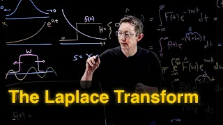
this video is sponsored by brilliant here we have a rectangular function and here is its associated

fourier

transform just a sinc function which is found through this equation here which makes this integral look scary especially for people who learn by first time, this is, of course, the exponential term. since it has I, but you know, let's remove it completely so we can see the geometric

intuition

behind this transformation. We can first expand e to at least I Omega T using Euler's formula by basic trigonometric rules, the negative in the cosine can simply be removed and the negative and sine function can be moved to the front as shown, just a little simplification, then I'll replace the ex menschell in the integral with that and lastly, we'll distribute the f of t. inside so we can divide this into two integrals, one with the cosine and not the sine where the right eye was taken out, so how can we visually understand this equation?

Simply take your function and multiply it by a cosine and a sine. curve both with the same arbitrary angular frequency and then find the area under both curves, which is what the integral tells us; those areas represent the real and imaginary component respectively of some complex number, since I is multiplied by one of those terms, the magnitude of that number is the magnitude of the Fourier transform on that specific Omega and the angle is the face as that we sweep the angular frequency and keep track of that magnitude and phase, however they can change, you get the full Fourier transform, that's pretty much it, we just find some areas put them in a right triangle and the magnitude and phase come from there and by the way the areas can be negative and integral senses so we need to think of this more like the unit circle where the phase can be positive or negative or greater than 90 degrees and so on, this will tell us if Some of those areas are really negative, which we will see later, but here let's go to an example.

I'll put the rectangular function back on top, but what we're going to do. is to multiply that by the cosine of Omega T and also the sine of Omega T, so we can see why this is the magnitude of the Fourier transform, which by the way is a function of Omega, make sure there's room on the screen is the most difficult part of this video, but I will keep the rectangular function plotted on both the left and right, but I will use points instead while the trigonometric functions will be solid. I'll start with Omega equals 3 cosine and sine of 3t, it looks like this, but since our rectangular function is 0 everywhere plus Then multiplying these regions together leaves us with the same things just cut off on the sides, as shown now, the Fourier transform says find the area under these curves and get the magnitude from there, since the areas under the x-axis are negative, so the graph on the right has an area of ​​0, the region of the left has an area of ​​approximately the point 6 6 and the magnitude of these is of course 0.66, the Pythagorean theorem is not needed when one side is 0, which means that Omega is equal to 3, the magnitude The Fourier transform is 0.66, so all we have to do from here is sweep Omega and keep track of those associated areas and this will give us the full magnitude of the Fourier transform.

By the way, notice that while I back up a bit, the graph on the right always has an area of ​​0, that will be the case even for a function symmetric about the y-axis because the positive and negative areas will always cancel when x sins any thing T, so we're really plotting this area as a function of Omega over all time in this case that's really all the Fourier transform is and let me also show you two points of interest, one is here at Omega equals 0 because this coordinate and it actually tells us the area under the curve, the reason why this is when Omega is 0 this here simply becomes 1, so we have the graph of f of T and the function on the right becomes zero regardless of what your f of T is, so we ignore that this means we're just playing the area of ​​f of T on the original curve, you can see that here the original rectangular function and the area under it, so let's move on to Omega is equal to 2 pi because it has a value of 0 on the magnitude graph, if you ever see a magnitude of 0 that means that if you multiply your original function by cosine or sine with that angular frequency 2 pi, in this case the area under both curves it will be zero.

This is where the graph on the left finally got enough negative area to cancel out the positive area and then as we continue to increase Omega, the area on the left oscillates from the network. negative to net positive while converging to zero, so we constructed the magnitude graph simply using real areas of real functions, we didn't have to really think about imaginary numbers to see the

intuition

here and just summarize all that with a slightly more complicated explanation . equation, let's say this is our f of T to find the Fourier transform, multiply it by the cosine and the sine of Omega T starting at Omega is equal to zero, which leaves us with just the function itself and y is equal to zero , then find the area under both curves. and use the Pythagorean theorem to get the magnitude and plot that point at Omega is equal to zero, then simply sweep Omega and keep track of that magnitude to create the Fourier transform magnitude graph for any Omega as 10, in In this case you will see that the magnitude of those areas are equal to the y coordinate in the bottom graph at that specific Omega and we see the same for negative values ​​of Omega, which means that this is the final magnitude of the Fourier transform and very quick about the phase, remember it was just the angle in the triangle with side lengths equal to those areas that we see here, if that phase is close to 90 like it is now, then the times cosine graph Omega T to the left has much less area than the Omega T 1 sinus on the right visually means that the length of the fundus is very small compared to the height.

Now I will show the actual phase graph which has a value of about negative 80 degrees at Omega is equal to 10, why is it negative low? Well, because that imaginary term from before, also known as the height of the triangle had a negative sign in front of it essentially we are in the fourth quadrant of the unit circle where negative 80 degrees is due to the negative Y value, then when I change Omega, we can see some intuition behind the face, like when it is approximately 45 or negative 45 degrees, for example, then the absolute value of the two areas is approximately the same, since it corresponds to a 45-45-90 triangle with two lengths of equal sides and if the angle reaches or approaches zero then the omega-t sinusoidal graph on the right will have zero or near zero area, essentially our triangle no longer has height, so when we have positive phase values at least between 0 and 180, this corresponds to a negative area for the omega-t sinusoidal graph, so in the end the magnitude graph tells you how large the areas are when combined, but in reality, when you simply apply The Pythagorean theorem, the phase graph, on the other hand, tells you relatively how big one area is compared to the other, as well as if any of them are negative, put them together and you get the full picture of the transform.

Fourier. Now let me ask what is the area under the full curve of cosine X from negative infinity to infinity. Well, I guess we can say it doesn't exist. because the area oscillates as the area moves away from the origin, it goes from 0 to 2 to minus 2 and does this forever, also H around 0, so that may not be correct, but we'll just call that infinite area 0, but Now, what about two multiplied cosine functions? I'm using two curves with very different periods, which makes for a strange looking graph, but even here the area will oscillate between two finite values.

In fact, I'll move to the right and I'll see that there are some regions with more green area and some with more blue area, but it keeps going back and forth, so again I'll call this area 0 as I change the period of one of those curves cosine, that area remains 0 in that oscillates and does not diverge even at this moment, where it seems that the area of ​​can diverge as we move, we still see that periodicity; However, once the two equations have the same period and only at this time does the graph rise above the x-axis. leaving us with infinite area, this is just cosine of PI . that by the cosine of Omega X and the sine of Omega Because the curve is always symmetric about the origin, even when the coefficients are the same, we still see that symmetry and zero area, so I'm going to completely ignore this graph for this one when Omega is equal to zero.

The associated graph has zero net area, which is a graph to start our Fourier transform magnitude, but even when we change Omega we will see the same thing as before, a total area that just oscillates, which we say is zero, but in Omega it is equals PI, the area suddenly jumps to infinity, which I' We will represent on the magnitude graph with an arrow and this only happens at Omega equals PI, the angular frequency of our original signal everywhere else, the Fourier transform, also known as the area, is zero, so this would be the final Fourier transform of the cosine PI X after taking that into account. even symmetry, this is the power of Fortier analysis, it sort of scans its original signal for sinusoidal functions, when it was on a wrong one the output was zero, but once it found the right frequency it gave us a short output infinite that said, hey, your original signal has a cosine of PI more complicated and apply the Fourier transform well, we can think of this as four separate integrals with each term multiplied by the cosine Omega T when there are no matches we get the zero area of ​​everything, but once our scanner finds a match we get that short infinite area and this will happen at different times, telling us now we have four sinusoids in our function, of course it's easy to see which sinusoids form this.

I mean, they're there, but if you gave them a square wave, for example, then it's not nearly as obvious; However, with our scanner we will find out. I'm just going to call the square wave F of T and to find what sign you sit on, we just sweep out the Omega term and look for infinite areas right now. Tomei is equal to zero, we are multiplying by 1, which gives us an area of ​​zero. equal parts blue and green, so it is not of interest as I increase Omega, this is still the case even here, if I were to scroll sideways I would see that all the blue and green regions cancel out, but in Omega it is equal to pi, we get a sudden infinite area. which means that we have found a sinusoid that forms our square wave that was hidden from us at first glance, but the Fourier transform found it.

However, this is not the only sinusoid in our function, we need to continue now. I am going to jump. around, so if we jump to omega is equal to 2pi, then the area will be zero. If you look closely, the blue and green regions cancel out, but when we go to 3pi there is a continuous pattern of more blue than green, so we get a negative infinite area, which means there is a cosine 3 pi T that also constitutes our function with that coefficient will be negative for the negative area. As I continue, it turns out that only odd integers multiplied by pi give us infinite area, which means that our square wave can be created by adding infinite quantities. cosine curves along with this pattern, which is the basic idea behind the Fourier series.

Now the last few minutes have been focused on having zero area or infinite area, which happens with periodic functions, but can we relate this to the previous parts when we got non-zero values? finite areas like is there something deeper in the fact that we get this continuous change in area for the rectangular function from before? Well, we could say that here at Omega is equal to 3, for example, our scanner found a cosine of 3t that forms the rectangular function. The only problem is that we should get an infinite area right now if that were the case because when we multiply the cosine 3t by itself we get that function with infinite area, but if we let that amplitude get infinitely close to 0, then we could get finite area at least whenwe treat this as a limit so in fact there is a cosine 3t which forms our rectangular function but it is infinitely small if we increase it I will make it three point one we still get a finite non-zero area which means there is also a cosine of three point one T in our function with an infinitely small amplitude.

This will be the case for almost all real numbers, although it means that we have to add an infinite number, a continuous spectrum of infinitely small sinusoids to make the rectangle. function and when it comes to visual intuition instead of peaks, we show a real continuous spectrum of values ​​that represent all the sinusoids that make up our signal and this animation that I have shown before highlights how that sum can create a real finite function now. I've made a whole video on the Laplace transform, but very quick since it's very similar, the biggest difference between Fourier and Laplace is the s and the exponent, but that really represents alpha plus I Omega, which I'll put into the equation and then divide the exponential as shown now, apart from having a zero as one of the limits, this is exactly the same as the Fourier transform with an additional term, so the Fourier acts as a sinusoid scanner.

Laplace scans sinusoids and exponentials in the same way. using areas here, let's say this is our function that starts at t equals zero. Laplace says x cosine and sine Omega T as before, but also including e to the minus alpha T, then find the area of ​​both to make room for these here. I'm just going to plot the cosine Omega T now we need two axes just for our Laplace transform inputs, one for Omega, also known as the sinusoids and one for alpha or Exponential, if we set both constants to zero, these are the areas and we write that magnitude about the zero point, point zero. now first I'm going to change Omega, which will move the point up on the imaginary axis and I'll watch how the graph changes once we get to Omega equals three and again it adjusts above the x axis so that the scanner has found the cosine of 3t. in the original function, but not really because we need an infinite area for that, there is no indication of anything special here in our output, but now I will change alpha or exponential and just eliminate the sine equation since the area is negligible. from here on out, but notice again how the graph changes once we get to alpha equals minus 0.5, there is no longer any decay and we get infinite area.

That infinite area now means that our scanners have found not only the sinusoid but also the exponential in the original f. of T just ignore the first negative and that exponential F, by the way, graphically these infinite areas are one of the only things we include in our graphs and they are represented with an X, so for those who need to understand zero pole graphs , just find their poles and look at the associated y and x coordinates because they tell you which sinusoids and exponentials are in your equation, pretty much all you need to know. We also plot values ​​that give us area zero, but those are not as important for our purposes.

Here, the reason the graph is so useful is because many systems, such as RLC circuits, masses on a spring, and just general control systems, produce sinusoidal and exponential outputs, so we need something more powerful than the transform. of Fourier to be able to analyze them again. I have a complete video. about Laplace, including 3D intuition, which I'll link below, but if you want to delve deeper into the applications we've seen here, I recommend checking out the brilliant series of differential equations. Your first course starts with the basics, but the second course is where you'll get into Fourier Laplace and much more that you probably didn't learn in an introductory differential equations course.

It really includes visual explanations, interactive exercises, and constant practice problems to ensure that you understand even complex topics fundamentally. You can put them into practice successfully. is an educational platform that hosts a variety of courses from differential equations to vector calculus to relativity and more, those looking to learn something new or simply relearn old material, plus the first 200 people to sign up will get a 20% discount on your annual premium subscription by visiting brilliant slash organization major CREP or clicking the link below and with that I'll end that video there if you liked it, make sure to LIKE and subscribe.

The social media links are below and I'll see them in the next video.