How to Create Impressive Interactive Excel Dashboard | Ultimate Excel Dashboard Ep. 1
Jun 05, 2021welcome to this first episode of my
tutorial series. In this tutorial series we sourced and
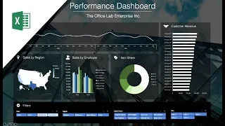
you see here. This dashboard is completely built in Excel and has so many features you wouldn't expect to have. possible in Excel, first of all, we have this beautiful, progressive layout on each element of this panel and with the slices at the bottom you can filter the underlying data from basically any angle you want. Each slice is connected to all the charts on the panel. The functions of these slices work perfectly together and you can select just one value per slice or dimension or if you want you can also do a multiple selection or filter and use another custom feature I
ultimate
excel
dashboard
tutorial series. In this tutorial series we sourced and create
d this amazinginteractive
Exceldashboard
you see here. This dashboard is completely built in Excel and has so many features you wouldn't expect to have. possible in Excel, first of all, we have this beautiful, progressive layout on each element of this panel and with the slices at the bottom you can filter the underlying data from basically any angle you want. Each slice is connected to all the charts on the panel. The functions of these slices work perfectly together and you can select just one value per slice or dimension or if you want you can also do a multiple selection or filter and use another custom feature I create
d is thisinteractive
info button that allows you to display u hide an information box that gives you additional information about the contents of the tile.
Then I found a great way to create multiple tabs within a tile that allows you to display different content in the same place where we have these beautiful tab buttons up there. and to top it all off, I created this huge foldable settings area that allows you to instantly modify the visual appearance of your dashboard. There you can choose between different gradient color themes using these simply beautiful radio buttons and with these modern toggle buttons you can enable or disable certain elements and functionalities in your dashboard, such as the tab functionality in our tiles or the information buttons, and If you disable and then re-enable items, they automatically reset to a predefined default state, which is pretty useful now in this first episode.

More Interesting Facts About,
how to create impressive interactive excel dashboard ultimate excel dashboard ep 1...
We will build a basic interactive dashboard that already has full filtering functionality. Then, in the following tutorials, we'll take a deeper, more holistic look at specific design topics. We will learn how to automatically update pivot tables and charts with changes. in our data and of course how to create these amazing top features have just been demonstrated so without further ado let's get started, since I received so many requests in the comments to make my files available for download I decided to launch a new website called Excel. Well, don't worry, there you will find the Excel files for this and my previous Excel, but they are available for free download and the good news is that I want to grow this website steadily until it becomes the number one platform for modern Excel skills and latest generation. techniques and resources so if you want to support me take a look and share Excel.

Find Calm with everyone you think might be interested and benefit from it and for everyone wondering what version of Excel or Microsoft Office I'm using in this video. Always use the Microsoft Office 365 subscription, which is pretty much the standard these days for most people I know and is required for many features. Use this panel. Microsoft is constantly adding new amazing and exclusive features, especially for PowerPoint and Excel, and with that version of Office you will be able to have all these amazing features available, so if you are still working with one of the older versions, I recommend upgrading to Office 365.

I personally would. got directly from the official Microsoft online store, probably the most reliable and fastest way to get the current version of Office. We'll link it in the description now for our basic interactive dashboard. The first thing we need is a good amount of source data. This panel will serve to measure the success of the customers of our hypothetical online store and for that we have a little less than 6,000. rows of data I generated automatically using a nice web script. I'm going to show you that script at the end of this tutorial series. Each row represents a customer transaction with all kinds of valuable information so that we have the date of the transaction.
The way this customer has been acquired organically through an ad or is a returning customer, then we have information about where this customer lives, which could be relevant for geo or micro targeting in our marketing strategies, then what product you bought and the respective price of that. product and the number of units and then based on that the revenue resulting from that transaction and we were even able to get information on the delivery performance i.e. whether the delivery was delayed or not and whether the customer returned the product for some reason and finally We asked our customers for feedback on the entire transaction and experience and they gave us some feedback on a scale of one to five.
Yes, that's what we got now. The first thing we want to do is put this data in a table that is really important for multiple reasons, the first reason is that it allows us to easily add new data below this table and then it will automatically be added to the table and the second reason is that then we can reference our dynamic data range by giving this table a name and simply referencing it. with that name whenever we want to use that data for one of our pivot tables and pivot charts, so let's call this table data table which allows us to start preparing our pivot tables and pivot charts for the dashboard.
At the beginning, we created a sales revenue line chart and for dad, we stopped inserting a pivot table, now we have to select the data and just to demonstrate to you, I will select the data range manually and you will see that it automatically detects this as a table that we just defined it has the data table name and that means. We can also just type the name of that table the next time we want to reference our data, since we want to see the revenue over time, we just drag the date field here down into the Pink box, as you can see, Excel automatically adds the years and the quarters field, which is quite useful in many cases, so now our Rose, our team, buys the quarters and this year; however, we don't need a fourth so we just delete it again and now we have everything we want, let's just open this up to show you and now we drag the income field into the value box which then shows us the sum of the income per year and by month in our pivot table.
Now let's insert a pivot chart based on a pivot table, so we simply click on that pivot chart button. right there and as you can see, by default, Excel inserts a bar chart if we group, you'll see that the pivot table is now connected to this pivot chart and for now, we'll first do a basic redesign for this pivot chart. We're going to change the chart type to line chart because we want to have a line chart and then we're going to remove certain elements that we don't need on our chart because in many cases, less is more.
Now let's format this quickly. axis, more specifically, we want to change the format of the numbers, so we change that category to currency and we want to have US dollars, there we go and set the decimal places to zero, that's exactly it now, that's all for now for this graph, so we can move on. Next up, which is the sales map chart for our sales map chart, we want to visualize our sales revenue by region to be more specific for us. For that we are going to insert a pivot table once again and this time we can write. directly the name, we don't even have to reference that datasheet, just type the name of the data table that we defined, click OK and that's it, and this time we want to drag the status field to the columns area, there we have our US states are beautiful and we drag the income field to the values area and there we have our income by region, as before we try to insert the pivot chart directly based on the pivot table and we have a nice chart of bars, the problem is if we try.
To change the graph type to map shot, what you see is that there is no map graph option, for some reason it is not there and we have to do this another way. One thing we tried is to directly insert a map, so now we get this alert. which says you can create this type of chart with data inside a pivot table. Select a different chart type or copy the data out of the pivot table. I don't know why this is, but Excel gives us some recommendations on what we should do. so we just do that, yeah, we copy the state names out of the pivot table type into the total revenue and now we can use the pivot data fetch function.
The pivot data fetch feature is a really cool feature because you can reference specific values within a pivot table. and then the cell value will behave as if it were inside the pivot table, so if you do any filtering on the pivot table in the original pivot table, this reference cell will simply behave as if it were in this pivot table and this filtering will be applied. to this cell too, now that we have created a dynamic copy of the pivot table, we can select the entire range and insert a map start directly and as you can see, this time it works from now on, it shows us the entire world and before for any data to be displayed. displayed, we have to accept that our data will be sent to Bing and that's it, now we have our data beautifully displayed, it automatically detected all the statuses correctly so we can continue to do some basic adjustments, which is, first of all, remove the title and then we do right click on the Sirius data and click on format data seriously and that opens the data series options area, there you have a field that says map area here we want to select only regions with data, now only the regions are shown with that, obviously, that's exactly what we want and just as a side note, this map capture is a very good example of a function that is only available in the latest versions of Excel, so if you use an older version it is most likely not available, max2 graphics will be available. beautiful donut charts in general, I don't really like pie charts from a visual point of view, on the other hand, donut charts can be designed to look beautiful if done the right way, like before starting, inserting a pivot table and referencing our source data. by the name we just gave our source data table, which is a table, look how easy it is and now we can't drag the delivery performance field into the Rose box, it shows us both and then we direct the field from income. in the values box, but this time we are not interested in the sum of income, which is the function that is applied by default, but we want to have the number of transactions there, we go to the field settings and change the function summarized by to count because that gives us the count of the number of transactions and now we have shown how many transactions have been late or arrived on time, since we want to show the percentage of on-time deliveries in the center of the donut chart, but we don't want use the native child tags as they sometimes change position with different values, we will use a fixed text field and to create the value for that tax field we simply calculate the percentage outside of the pivot table, then select a cell. inside the pivot table and we insert a pivot chart by default it is a bar chart again so we will change the chart type to tall and in the pie category we have the donut option here we go first we remove the title and then we have To make a quick adjustment to the pivot table with greater precision to the order of use of the well because what we want is the good value.
Timed trading in this case starts at 12 o'clock and then goes clockwise to scroll on our donut charts. we can do it by simply changing the sort order of the rows to perfect dis caning that's all for the chart now we just need the chart label, the percentage label and for that we are going to insert a text box now in this text box which We don't want to have a static well like you normally have in text boxes, but we want to have a well based on a cell reference and for all of you who don't know how to do this, it's actually pretty easy, just select the box. text, but then instead of typing directly into that text box, you click on the formula bar up there.
Now we can place a normal cell reference as we would any other cell. Now we just adjust the font size and tax. alignment and that's it for this chart, for the rate of return donut chart, it will be more or less the same procedure: we start again by inserting a pivot table that references our data table and this time we drag the return field to the row area andthere let's have both of us use yes um no and again direct an input to the value box and change the summary function to count because we're still interested in a number of transactions before we insert the pivot charts that we don't want to forget to calculate. the percentage value again for our text label and this time we will calculate the wrong value, so the return rate, obviously the number of returns is something we want to be as low as possible, change that to a pretty good percentage and now we can't insert. our pivot child likes before changing the chart type to donut type again, there we have it this time, the order of using the actual pot is already correct because we would like there to be no returns, the good value remains the one that starts at twelve o'clock clockwise and yes, the nodes insert the text label and reference the percentage value that we just calculated now let's just adjust the text size and let's do it again here we go and the alignment of the text and that's it with the preparation of these donut charts I admit that they don't look pretty at all right now, but I promised that they will be when we finish with the layout of the board, the next chart will be about the type of customer acquisition and for that we're going to use a brand new type of chart which, by the way, is quite popular with a lot of people in the business world and, again, is only available in newer versions of Microsoft Office.
You guessed it. I'm talking about the waterfall chart again, we'll need a pivot. chart, so let's insert one and reference our source data like before we continue and this time we're interested in the customer acquisition type, so we'll drag it into the row box and drag the revenue field into the row box. values and once again we want to have the number of transactions so we will change the summary functionTo count beautiful now let's insert a perverted chart for this pivot table and change the chart type to waterfall type there it is and what is that oh man, It doesn't seem to work either.
It's the same message as for the map chart before it. recommends copying the data out of the table, um, yeah, so I guess we have to do that, I hope they fix that, but anyway, the nice thing about this is that now we can adjust the order of these row elements of the way we want. in a way that wouldn't be possible within a pivot table, so that's good, yeah, and then we'll use the get pivot data function to reference our pivot data values again and this time we also have to include the total in the The previous charts we didn't include that because it wasn't necessary, but for the aqua charts it is necessary because it will be a bar that summarizes all the other bars that you have left and now that we have our data set up, we can insert the waterfall chart, here we go, let's do it a little bit bigger and let's remove these title and lachen elements and this now, one problem with the setup of this chart so far is that the totals bar is not set up as a totals bar, it's just another bar. above the others to fix that we just right click on this specific data point and click on format data point and there we have the satis total option just say yes do that and there we go this is what our should look like waterfall chart if you redo it, it's just another bar and this way it works totally beautifully.
We are almost done with preparing the graph, there is only one step left to finish the last graph. will display customer satisfaction divided by product, let's insert another pivot table and this time Let's create a two-dimensional pivot table, we start by dragging the Customer Satisfaction field to the Pink box and if you look closely at the row we will use, you will see where it is important to have these numbers from one to five in front. the description because that guarantees the correct order of these row elements. As a next step, let's drag the revenue field into the value box and set the summary function to count again because we want to have the number of transactions and the four-column box that we want again. we have the product field there and now we have our beautiful two dimensional pivot table, this allows us to insert a pivot chart and now we change the chart type to a normalized horizontal bar chart.
It is called 100% stacked bar chart in Excel. Wow and I see that we have to change the product and complete the customer satisfaction and as you can see we can do that directly in the pivot chart which is great now we want it to start with product one at the top so let's change the sort order to go down and remove those awesome access lines, that's it, we've done it, we've just prepared all the necessary dynamic charts for our dashboard, now let's move on to the fun part, booyah, as you can see in the basic layout from the panel I already prepared. a stylish background and a beautiful gradient that I designed for our dashboard graphics and slices, but don't worry, I will cover how to prepare all this in the next episode of this tutorial series, since it takes a little time and I want to cover different variants of design.
We decided to make it a separate video. Now let's fill this beautiful bow tie design with some life and forever we want to insert a header by inserting a tax box by changing the tax size to 32 and then just type whatever name you want to give our panel. in our case we call it customer success panel because that's what it is, just resize it and right click on it to format this shape, let's just remove the fill and remove the line and then change the color to white and the overlay to Center. and the middle and now we can finally reposition it in a good position, perfect.
Next we want to insert titles for our four beautiful mosaics and what are we going to need? A background. We don't just want to just add titles but we want to put. them inside a nice background box for which we use a rounded rectangle and set the roundness to maximum, make it a little bit bigger and then change to fill to white and remove the line and then change to transparency to cat5, let's make it a little less, let's make it at 80% so it's very close to the background but still differentiated from it and yeah, I think it looks pretty good now we duplicate this three times and place it on the other three tiles, which is the first one and then the second. one and we always try to find exactly the same relative position within the tiles.
The best way to make these minor positional changes is to use the arrow keys and there we go, now we have all those nice title background boxes, so let's put some content in there. Before placing the actual titles, we want to insert some attractive icons and for that we will use the built-in icon library which is such an amazing feature in Office 365. I can tell you that I still remember in my last dashboard videos I received many requests about where I got these amazing icons and this built-in library is the answer. Microsoft has been steadily expanding this library of icons over the past few months, so now with the current version of Office link in the description, you have a huge amount. of attractive icons available now for our purpose, let's select these four and insert them there, we have them, let's start by changing the color to white and since we have all four selected, we can resize all of these at the same time. maybe it's a little bit bigger, let's do it, oh, point three should be perfect and now let's put them inside these transparent background boxes.
The reason I really prefer these built-in icons over externally sourced icons is that they are flat, look beautiful, and the best. The important thing is that they are fully customizable within Excel, so for example if you want to adjust the color of one of these icons you can easily do so within Excel and change it to the color you want, but that is not the case if you use an external source like a website for free icons for example, now that we have our icons in place we want to add the header titles, for that we simply copy the header title, drag it down and change the text size to 14, then let's change the size of this text. box and change the text there for the first time to call it sales because there we will have two sales revenue line charts and the sales revenue map chart and we adjust the size of this transparent background box to fit the length of our title text now let's copy that title to the next tile and change the text accordingly, this tile will be called deliveries because there we will place our two donor boxes that cover delivery performance and return rate.
Okay, now let's copy it another time. for the next tie, which will be about customer acquisition, customer acquisition, obviously, like one or two words longer, so we have to make the text box bigger and then in the same way, we have to make the text box bigger. background too so it looks good. and then we'll copy that title to the last link, which is the customer satisfaction tile, we'll also expand this box and that's it. Now we are ready to insert the dynamic charts that we just prepared a few minutes ago. Let's start with the sales revenue line chart, we cut and pasted it here and right now it obviously looks like a misfit from a visual point of view, but we have to redesign it in just a few simple steps to make it look beautiful, we begin.
By making use of this predefined chart layout which you can find in the chart layout tab and then we are going to format the chart area to remove the padding and border, we will resize this chart to fit there approximately and we have to Please note to leave some space on the right side because there we want to add the sales revenue map graph later. A big problem here is that the proportion of the time axis with its labels is more than a third of the entire chart area. and we want to have more space for the actual content of the chart without losing the readability of the chart, which means we still want months and years to be displayed for this axis, so what we're going to do is first reduce the text size of these .
Now we have labels that are displayed every month there, but if they were only displayed every two months, the readability would be just as good, so let's open the formatting access section on the right and in the XS position we select the check marks and then the important part in the tags section there we deselect the multi level category tags option which removes the year tags for a second but then when specifying the interval unit and we go with two here the years appear again and the whole axis area is much smaller now, now there is just I would like to add a small detail, for that you have to click on the data seriously and there you can change the line layout to a gradient line, then delete those intermediate colors, change the right color to red by default, the angle is 90 degrees and now. if we take it to a 50% position, the effect that you get is that the lowest utilization of the pot will be colored in this red gradient, so the bad values will be slightly red and I think it's just a beautiful visualization of the values bad or good if you like, but for this, but I decided to play with different shades of red, we continue by inserting the second shot, which is the sales revenue map graph, we cut it and then we paste it here and the first thing we want to do . is to format the chart area by removing a padding and removing the border line, then I decided to also remove the legend because we don't really need it if we style it the right way and then resize it and place it in a good position. where it suits you perfectly in terms of color, the adjustments will be quite simple: just right click on the map and click on format data series and in the format section we change the color of the highest value to red and the value lower to white and That's it for this chart, the next two dynamic charts will insert attitude ring charts and will require a little more effort, but in the end they will look amazing.
Alright, so we'll start with the delivery performance graph and we'll cut across both graphs. and the text field label and paste it here, you will directly see a problem because obviously this reference is not working, nothing appears there and the problem is that we need to manually add the datasheet name there, so quickly do that boom of the delivery performance donut and there you'll see the number is, here's how to fix it, we're going to remove that legend and then we're going to resize this area of the chart to 1.5 and 1.5. Now let's right click on it and click format. chart area to remove the padding and border line, then we want to change the color of the data series, quickly drag them down to see them better,we click on it and change the fill to a solid fill which will make both data points white and We also set the border to a solid line and for our second data point we actually wanted it to have no fill so we click that specific data point and we set it to no padding and since we already set that border to a solid line, now it looks like this, which is beautiful and finally we reset the ring hole size to ID now let's say 85% and that gives this graphic its final appearance.
Now for the label we want to start by also removing the fill and the line by changing the color to white. and setting the text size to let's say 28, then we resize this text box and place it a little bit in the center of this beautiful donut chart, not exactly in the center because we want to place another label just below that gives us more information about what The percentage number actually means correct, so we insert another text box and then specify this percentage by typing on time, so now it says okay, we have 67% of our deliveries on time.
A good tip at this point is for the number tag to enter the descriptive tag below. it should be about the same width to give it a clean look and right now they're both not perfectly centered together, so let's move them up a little bit. I thought it would be a great idea to not leave the space below that chart unused, so we decided to add additional information about the target value we want this specific value to be for. We begin by inserting a line to visually separate this additional information from the chart. We make sure that this line is perfectly horizontal, which it obviously is, and we change. the color to white we add the width to a point then we reposition it and try to make it perfectly centered by selecting the chart area, the line and the line in Center and then we just copy this descriptive label, place it here and then change the send a text to aim for 70% because we want to hit 70 percent on time with our deliveries, so one thing, let's make our goal bold to stand out a little bit and that's it for this beautiful donut chart, okay, Now let's replicate this exact redesign. process for the other donut chart, the rate of return donut chart and for that we will cut the chart plus the tax field label and paste it on our dashboard sheet and again we have to fix the problem with our tax field label text and broken cell. reference so let's insert the name of the rate of return ring sheet into that reference and now it works great again so we can continue by removing this legend and formatting the chart area by setting it to no fill or line and then we will change the size. at the same size as before 1.5 and 1.5, just drag it down to see it better and now let's change the color of the data, make it all white for the moment and set it to solid line and then let's remove the padding for this specific data point exactly. so let's take a quick look at what is the width of the line here set it to one point and let's do the same for this line as well and now we just need to adjust the ring hole size and set it to 85% perfect just put it in quickly . over the other donut chart to check if it has the same proportions and that is the case so we can continue with the label again for the label we want to set without padding or line.
Make the text white and set it to 28 exactly. Make the tax feel a little smaller. Place it right there. Now we need to make sure both rings. The graphics and labels are all at the same height. You can do this by lining them up or simply overlapping them and then using the arrow keys to move them to the right. That's what we'll do. You can see it well. Do the same with our number label. Perfect, now. just copy these other three elements and overlay them like this perfect and move them to the right and that's it, that looks pretty good now we just need to change the text content so we'll change the trigger time to returns because we have 10% performance and to Our target global year will be set at 8%.
We're really ambitious, yes, and that's it for these donut charts, don't they look beautiful? Now let's move on to the waterfall chart. Let's start by going to the Custom Acquisition Waterfall Tab, cut the chart and paste it into the dashboard sheet. There it is, let's make it a little bit smaller and format the chart area because again we want to remove the padding and the border exactly and then we'll get rid of this. y axis because we already have the values in the labels above the bars, that should be enough and then we'll try to make it fit perfectly in this tile, let's change the color of these data labels to white and then I'm going to change the format of these data labels data, first of all, the position of the label, let's enter it and for the numbers forward and we will change that to a number with zero decimal places exactly like this for our labels at the bottom.
I'm going to change that color to white. make it a little bigger like this, perfect, and then let's move everything up a little bit so that the graph line, the access line, is about the same height as the other two lines on the left. Now we can deal with the bars. first of all we want to change the border of these bars make them one continuous line change the width to a point and the color to white exactly like this and now we are going to take care of the fill, we go there and change the Fill all these bars with gradient fill, then we will delete those middle colors and then we'll change the colors, so for the one on the left we want it to be white, yeah, and for the one on the right we want it to be purple, you'll find it.
Down there the standard colors are exactly like this and now it's very important that we set the transparency for the purple to fifty and for the white to fifty as well and this gives us this beautiful look. Now he simply changed the angle to 120 degrees to rotate it. a bit and something quite common for waterfall charts is that the total bar has a different color than all the other bars, so let's change that width to this red and this gives us this beautiful gradient style for the entire chart, eventually we can move forward. to our final graph, which again will be our customer satisfaction horizontal bar graph, we're going to cut and paste it onto our dash sheet and make it somehow fit on that tire for now, the first thing we want to address is this legend because you want to reposition it and bring it to the bottom instead of the right side because that makes all the space used more efficiently and let's just change the text size to 7 for this legend and then we're going to format the chart area, set it in no padding or line, click on one of these data series and adjust the width of the space between the bars, something close, well I would say something close to 100 should be fine, yeah, well I decided to go to the tab layout and add a chart element.
We already removed that, but I think it could make sense, so we added vertical grid lines here because then we don't have to put labels on the bars because you somehow know which percentage line you are on. I just want to change the color of these to something slightly gray, maybe not that one and let's reduce the width of that, then for these product labels, we'll change the color to white and do the same thing for the percentage labels there exactly on that moment. The next thing we want to do is, as before, for the water flow diagram, we want to add lines to border the bars and we need to do this for each data series that you see, each color is considered separate. data series that you and I just looked at, of course, I want the legend text at the bottom to also be white instead of that dark gray and I think maybe we should reposition it slightly and resize it. this graphic to make it more visually appealing.
The problem I see. What comes up now is that our vertical grid lines somehow disappear, but we can easily fix this by manually setting the unit interval of the major axis. There we go to 0.2 and there we have our 20% steps again and for the grid lines themselves, I think it might make sense to change. Something might not be really happy with it now, maybe change the color or let's try to play with the transparency like this. I think it's pretty good, let's leave it at that now. The last thing we need to deal with on this chart is the color of this serious data.
I decided to make it a gradient style, a gradient fill for all of these bars, always with slightly different colored tubes, so for bad, serious and very low and low, we will use some red tones for you and for the ones in the middle we will use a combination of white and a little bit of gray and then for the good ones, for the high and very high satisfaction that you have, we will use some shades of green for those wondering some of These colors are normal theme colors or standard colors and then some others are recently safe colors or something that I customized with the color tool and that's why they are still saved in the recent colors down there and now we have completed the next main part for this basic version of the dashboard, the last thing we definitely need to add because we want it to be a fully interactive dashboard, is to use beautiful interactive slices for our pivot charts and you might be wondering why this guy says beautiful slices, because Yes you are.
If you're familiar with Excel's PivotTable and Chart sectors, you know that the default and even the fallback are starting to look not very good, quite dated, and definitely wouldn't fit into this; that's what we just created for, but don't worry, I prepared a beautiful modern and state-of-the-art Cutting Design that fits perfectly on this board so that it looks beautiful as promised, but before we talk about the cutting design, first we have to insert it, so let's select one of these pivot charts, click on the Insert tab and there. we have the segmentations now, this opens this popup window where we can select which dimensions we want to have divisions for, we will select the type of customer acquisition of the product by years and we will indicate that these are the four divisions that we want to have and there they are.
They're not really beautiful, anyway, let's put them next to each other so we can see them well. Now the first thing we need to do is select the four slices and right click on them and then go to the slice settings and there see the option to hide elements without data and that is something we definitely want to do. I definitely recommend it because, for example, in the years tab you see all these unnecessary fields that we don't need and that will hide them and now that we have the four sectors selected, we are going to connect them to all the other pivot charts because currently they are only connected to our fancy line graph and we have to click report connections.
Well, it looks like we can't do that for all four at once, so we have to do it slicer by slicer, we right click on the first one and we're going to report connections and that opens this popup window where we just select all of these pivot tables, you'll see which are pivot tables, but I mean these pivot tables are directly connected to these pivot charts, so it's basically the same thing and now we just do this three more times for the other three slices for a product segmentation for acquisition segmentation of customers and finally for our status segmentation, here we go and now we can fully concentrate on cutting a design as I told you before, I already prepared a custom modern and advanced cutting design and I think many of you are interested in how to do it.
This will be covered in detail in the third episode of this
ultimate
board tutorial series. will show you everything like the overall style, this beautiful hover effect and the stars of the selected and unselected elements, but for now let's enjoy its beauty and make it fit into our black crop area so that they fit perfectly, you need to use the options you have above in a slicer tab that allows you to define how many columns you want to have and what the height and width of these columns are, so for our first slicer we are going to make it two columns and slightly adjust the proportions of this slicer for the second segment it makes sense to convert it into three columns since we have five elements in total there and for the third we do it in columns again and you always have to play with the proportions of these segments to make everything visible because if there is not enough space it will simply cut words, sometimes it can't be helped, but you need to make sure that at least most of the content within these sectors is completely visible and if not, that it is still understandable and that's it, friends.Let's take a quick look at what ourfinal panel is able to do. It allows us to divide our large amount of data into basically any dimension we want, so that, for example, we can filter our dashboard shots by individual years. We can even apply multiple selection. Multiple years can be selected, like here we have 2018 and 2019, as you can see, and we can apply the same for product portions, so for example, let's split our data into products two to four or alternatively three to five. Everything is possible with this basic. Excel interactive dashboard and just as a summary, what makes this dashboard really powerful is that all of these slicers are working together, which means that if you filter within one slicer and then also filter within another slicer, all of these filters are active at the same time and that allows you to split your data to get even the smallest data cube within your big data cube.
I hope you liked this tutorial again. I recommend visiting my Excel website. Find calm. There you will find all the files of this dashboard tutorial series for free download and also you will find a lot of valuable Excel knowledge and resources there so just take a look and I appreciate anyone who shares it and spreads the word and that's all for now , don't forget to subscribe and don't miss it. in the next amazing video in this tutorial series. Greetings.
If you have any copyright issue, please Contact