Analytic Continuation and the Zeta Function
May 12, 2024Before I start today's video, I wanted to tell you that I have another channel that I started recently where I talk about sudoku and other related pencil puzzles. If you are interested, below is a link to
zeta
mathematics. puzzle channel I stream there once a week, so if you want additionalzeta
math content, feel free to check it out. Hello and welcome to zetamath. Last time on zetamath we told the story of how Euler realized that, just like a polynomial, it was possible to factorize thefunction
. The sine of x as a product in terms of its zeros led him to discover the fascinating identity The sine of x is equal to x multiplied by this product when n goes from one to infinity of one minus although fascinating in itself Well, we use this to motivate Riemann's discovery of a similar product formula for the zetafunction
in terms of its zeros.
That product formula looks like this zeta of s is equal to e raised to some power divided by s minus one times the product between the zeros of the zeta function of one minus s over alpha multiplied by some power of e we talked about at the end of the last video about how Riemann used this formula to derive an explicit formula describing the distribution of primes. Riemann's key idea here was that in order for this product formula to work, he needed to view the zeta function not as real number inputs but as complex number inputs.

More Interesting Facts About,
analytic continuation and the zeta function...
Today's video marks the beginning of a series in which we will seek to motivate the study of complex numbers and understand them. The Euler and Riemann formulas for the sine of x and zeta of s are better. My goal is to convince you that, in some sense, as soon as we define a real function, we can already evaluate that function on the complex numbers, like this. To avoid having to ask what the sine of 3 plus 2i or the zeta of 5 minus 2i means, we can simply assign values to them. Today we begin our story with Bombelli, who was perhaps the first to notice that when contemplating complex numbers.

He might provide some interesting information about real numbers to start with, let's remember the quadratic formula which gives the roots of a quadratic equation in terms of its coefficients. This number under the square root is usually called the discriminant of the quadratic equation, often denoted with a capital letter delta and this discriminant helps tell you the nature of the roots of the quadratic if delta is positive that tells you that this quadratic has two real roots if delta is zero that tells you that this quadratic has exactly one real root with the so-called multiplicity 2. If however, delta is negative, then this formula gives us a square root of a negative number and that tells you that the quadratic It has no roots or, if you prefer, it has two strictly complex roots.

The quadratic formula was known even to the ancient Babylonians, but it was not until the year 1500 that Cardano discovered a similar formula for the roots of a cubic polynomial. What a mess. You can immediately see why this formula was probably not taught to you in school and I want to give you an example just to show you that This formula is actually a little worse to use in practice than it might seem at first. I'm going to start with the example x cubed plus 6x minus 20 and we'll use this formula to calculate a root. Plugging in 6 for p and negative 20 for q we are left with the cube root of 10 plus 6 times the square root of 3 plus the cube root of 10 minus 6 times the square root of 3.
After some thought, you can convince yourself. that the cube root of 10 plus 6 times the square root of 3 is actually 1 plus the square root of 3. How do we know that? Well, just cube 1 plus the square root of 3 and make sure you get 10 plus 6 times the square root of 3. square root of 3. Similarly, the cube root of 10 minus 6 times the square root of 3 is 1 minus the square root of 3. By substituting those cube roots into our formula we find that 1 plus the square root of 3 plus 1 minus the square root of 3 is a root of our original cubic, that number, of course, is just 2.
So It is easy for us to verify by substituting 2 into the original cubic that the formula gave us something correct because 2 cubed is 8 plus 2 times 6 is 12 minus 20 is zero, the cubic that Bombelli found was x cubed minus 15 x minus four if If you apply the above formula, then the root of this cube you get is the cube root of 2 plus the square root of negative 121 plus the cube root of 2 minus the square root of negative 121. Our experience with the quadratic formula suggests that these roots squares of negative numbers appearing in the formula would mean that this cubic has no real roots.
In fact, this is what Bombelli also expected, except that Bombelli already knew that x equals four was a root of this polynomial, did this mean that Cardano's formula was wrong? What was happening? What Bombelli noticed was that if you simply pretended that taking the square root of negative numbers made sense, even though everyone at the time knew it was obviously absurd. so you could see that actually 2 plus the square root of negative 1 cubed was equal to 2 plus the square root of negative 121 and 2 minus the square root of negative 1 cubed was equal to 2 minus the square root of negative 121. these numbers for the cube roots in the formula, then the formula tells us that 2 plus the square root of negative 1 plus 2 minus the square root of negative 1 is a root of this cubic but of course that number is just one form complicated to write 4 which is what bombelli expected, in fact if you take a step back in this example the square roots of minus 1 behave exactly as the square roots of 3 behaved in the previous example the fact that this square root is of a negative number ends up not providing any significant difference in how this all works, Bombelli certainly didn't think of himself as discovering a new number system when he did this, he simply thought of himself as finding a shortcut through algebra that was able to get the answer. to the question that wanted to get out of the formula they already had, but once Bombelli opened the door to thinking about square roots of negative numbers, mathematicians found many places where thinking about them helped them answer questions they already had and that in They themselves implied nothing. about the square roots of negative numbers, as usual in this video, we are going to visualize the complex numbers on a plane like this with the real numbers on this line and the strictly complex numbers on this line, for example, 3 plus 4. i in this image it would be somewhere around here we will also see graphs of real functions like the sine of x that appear in r2 to avoid possible confusion we will always show the complex plane with these grid lines and r2 without them the task What we have before us is take a function like the sine of x or the tangent of x or e to x that is defined somewhere on the real line and find a way to evaluate it meaningfully outside the real line.
The key word here is significantly. because apparently there are many ways to define this function outside the actual line, for example you could define the function to take the value 0 everywhere not on the actual line or just say, ignore the complex part entirely, just take the sine of 2 if someone asks you about the sine of 2 plus 3i, for example, but if we want to be honest and meaningful about it, I want to convince you that there's really only one way to do this and I'll call this process thickening E The goal is not to immediately define this function on all complex numbers.
My goal is to simply extend this function a little bit beyond the actual line, so visually what I'm thinking here is to take a function that is defined only on the actual line. line and then just blur it a little bit so that it's defined a little bit on each side and then once we do that, we can go a little bit further and a little bit more and eventually end up defining the feature across much of the line. complex plane The key observation that drives this process is that if the function I start with is a polynomial, then I can extend it to complex numbers simply by using the regular operations of addition and multiplication of complex numbers, for example, if I start with the function f of x is 15 plus 42 i, this really only works for polynomials, although I can't say, well if someone asks you to plug 3 plus 2i into sine, just take the sine of 3 plus 2i, it doesn't help at all in that case, a convention What you will often see is to denote a function in which you intend to connect real numbers with the variable x and a function in which you intend to connect complex numbers with the variables z or s, this is the reason why most of the time, when you see When people talk about the zeta function, we see it expressed as zeta of s instead of zeta of x, so in terms of this convention, what we've basically said is that if we want to take the real function f of x equals x cubed minus 2x and turn it into a complex function, all we can do is replace the x's with the z's.
The reason this is important is that, in essence, every nice function is already almost a polynomial. If that sounds strange to you, essentially every time you think of a McLaren series or a Taylor series for a feature. What I do is take a function and write it in a form that is pretty close to a polynomial as a first example. I want to start with the sine sine function of x, as we discussed in the previous video, it has the Maclaurin series x minus x cubed in three factorials. plus . It's not very easy, but what I can do is plug it into the first one, however many terms I want, and then stop here on this table.
I'll show you what happens if you connect it to just the first term, the first two terms, the first three terms. and so on, and what we see is that if we plug this into not so many terms, we already get that it is close to the value of half that we expect for the sine of pi over six, we can actually see that this happens for all real numbers . Right away, if we look at this sine graph and then plot the partial sums of the Maclaurin series over it, here is x and x minus x cubed over three factorials and x minus x cubed over three factorials plus x to the fifth over five factorials and so on.
Note how quickly the partial sums hug the graph of the sine of x. So how do we evaluate sine into a complex number like 3 plus 2i? Well, we just do the same thing: we plug 3 plus 2i into each of these partial sums and look at the values and we can see that these partial sums converge pretty quickly. Just by looking at these values we can conclude that the sine of 3 plus 2i must be some number close to 0.53 minus 3.59 i in the case of the sine of x, it is actually the case that we can calculate the value of the sine of any complex number by simply plugging it into the partial sums of our maclaurin series and waiting for it to converge unfortunately the overall situation is a little more complicated to see what goes wrong let's look at this graph of the real tangent function of x note that this does not is the complex plane, it's just our typical r2 where I graphed y is equal to the tangent of x now I'm going to graph on top of this the partial sums of maclaurin series looking at these partial sums we see that they provide better and better approximations of the tangent of x, but just in this narrow band even for real inputs my maclaurin series for the tangent of x can't tell me what the value of the tangent is supposed to be of x here, the reason for this is that the graph of the tangent of is to have an asymptote so what happens is that our polynomial approximations of the tangent of x do the best they can and it turns out that the polynomial approximations can never exceed these two asymptotes.
These points on the graph that cannot be approximated by polynomials are often called singularities. If we try to enter complex numbers here like we did before, we will find something similar if I plug in a complex. number that is close enough to zero as one plus i, then we see that the partial sums converge just as they did before with sine, if we try to plug 3 plus 2 i into the partial sums, this happens, wow, no matter how many terms of the partial The sum I write just isn't getting better. Summarizing what we know so far, the Maclaurin series for the tangent converges in the complex plane at this red line.
We also know that it converges to one plus i, which I will indicate by putting this point in red. then we saw that it diverges at point 3 plus 2i, whichI will indicate by putting this point in gray. Let's try a little more on i. The series converges at 1 minus 2i. Diversify. Let's try many more examples of this image. I assume that the points on the complex plane where the Maclaurin series converges for the tangent take the shape of this disk, so we have made two examples sine of x whose graph looks like this where it turned out that we could use the Maclaurin series in 0 to evaluate the function anywhere in the complex and tangent plane of x whose graph looks like this where it turned out that we could only evaluate the function at some complex numbers close enough to the origin.
I'm going to show you a third function here is the function. f of x is equal to 1 over 1 plus x squared, which do you expect to be the sine of x or the tangent of x? Seeing that this graph has no asymptotes, it would be reasonable to expect this function to behave like the sine of x, but as you can see as I graph the partial sums of the Maclaurin series, it only converges on this interval, remember this red.The interval in the graph on the left is this red line in the complex plane on the right, like I did with the tangent of x.
I'm going to insert some random numbers into the Maclaurin series of 1 over 1 plus x squared and mark those where it converges and those where it diverges, why is this happening even though we see that our function has this nice smooth graph? If we broaden our view here and think about the complex plane instead of the real line, we can see that the tangent to x has asymptotes here and here, on the other hand, 1 over x squared plus 1 actually has asymptotes at i and minus i because if we substituted i or minus i into this function we would get one over zero and what we see happening here is that the region in which the Maclaurin series converges starts at zero and then grows symmetrically around it until we reach the first singularity.
What I find particularly notable about this is that the asymptotes of one over one plus x squared at x equals i and x equals minus i stop the maclaurin series from converging even on the real numbers beyond -1 and 1. In this way, the behavior of this function in the complex numbers is affecting the way the Maclaurin series behaves in the real numbers. It is a general fact that for any reasonable function its Maclaurin series will converge within a circle whose radius is equal to the distance to the singularity closest to zero in the complex plane. The reason the sine of x example above didn't have any of these problems is that the sine of x function is an integer. which means that it has no singularities anywhere in the complex plane the zeta function of s that interests us most has a singularity here at s is equal to one this appears as an asymptote on this graph of zeta on the real line something else apparent in However, this graph is that the zeta function of s defined by this series doesn't even make sense for s less than one, therefore the zeta function of s has no mclaren series.
Fortunately, our cure here is relatively simple, we just need to change our perspective from thinking about things centered at zero to thinking about them centered at some other point. You may remember from your calculus classes that this idea is generally known as the Taylor series instead of writing the Maclaurin series which has the form of zero. plus one x plus two x squared and so on, instead we are going to write a series of the form a zero plus one times x minus x zero plus a two times x minus x zero squared and so on where we have We change our center now from x is equal to zero to x is equal to x zero in a McLaren series if x is very close to zero all the terms are small because the powers of small numbers are small in a Taylor series all the terms are small no if x is close to zero, but if x is close to x zero because that makes x minus x not small, what is now true is that if we start at any point x zero on the real line we write the Taylor series at that point , then that Taylor series will converge. in the complex plane in a circle around x zero whose radius is equal to the distance to the singularity closest to x zero in the complex plane as an example let's look at the tangent again the asymptotes of the tangent are here in pi over 2 3 pi over 2 and so on, let's try to evaluate the tangent of 3 plus i.
I definitely can't use the Maclaurin series for the tangent to do this because 3 plus i is further from the origin than this asymptote at pi over 2. However, if instead we take the Taylor series for the tangent of x centered at x equals pi and then we plug 3 plus i into the partial sums, we find that it converges quickly and we conclude that the tangent of 3 plus i must be approximately negative 0.06 plus 0.76 i, so here's a summary of how we start with a function that is defined on the real line and obtain a function that is defined at least around the real line in the complex plane, that is, at each point on the real line where our function is defined, we take its series of Taylor and we use it to define the function in a circle around that point we do this at each point on the real line and thus we end up defining our function again at points close to the real line remember that calculating the Taylor series only requires calculating the derivatives of the function and for that we only need information about the function on the real line and from that we can define what the values of the function should be at the points of the complex plane, essentially we can think of it as if those values of the function on the complex plane they were there.
All along we had not really thought about looking at them. A key feature of this method is that it frees us from thinking about what any of these functions mean on the complex numbers, so we can use this method for any function defined on the real numbers and simply extend it to the complex numbers as we have discussed. Here, this is all very strange, but a word that mathematicians like to use to describe this is to say that complex functions are very rigid, the values of a complex function on even just a small piece of the real line is enough to dictate the values of that function anywhere else.
One way to say it is that it is not possible to change the value of a complex function here without also changing it here in each value of a complex function. At each point it carries information about each value of the complex function at all other points. Ultimately, it is through this rigidity of complex functions that the zeros of the zeta function end up dictating the distribution of prime numbers, but we have a problem. is that so far we have only managed to extend our function to points close to the real line, so, for example, if we try to calculate the tangent of 3 plus 2i using our method, it will fail no matter where on the real line we start because tangent asymptotes prevents us from using this method to define the tangent more than a distance of pi over 2 from the real line, although the answer to this problem is surprisingly simple, that is, if I want to know what the tangent of 3 plus 2 i Can I start here at pi which defines the tangent inside this disk? 3 plus 2i is here outside the disk, but 3 plus i, as we saw before, is on the disk, so we write the Taylor tangent series at this point, which Now let us define the tangent anywhere inside this disk that includes 3 plus 2i and that will allow us to define the tangent of 3 plus 2and now that all sounds so natural you may not even realize that what I just said requires us to take the derivatives of functions on complex numbers, which initially sounds pretty scary, the reason we need those derivatives is that our formula for the Taylor series of a function is the sum as k goes from zero to infinity of the kth derivative of f evaluated at x zero over k multiplied factorial for x minus in 3 plus 2y, but this is where we get to one of the best parts about the way we've created complex functions from real functions.
Let's get the derivatives of these functions in complex numbers for free. Because? Well, ultimately. because we know the power rule, so for example, if I want to know the derivative of the sine of x at 3 plus 2i, then what I do is take the derivative of x minus x cubed over 3 factorial plus x to the fifth over 5 factorial and so that just requires the power rule and I get one minus x squared over two factorials plus x up to the fourth factorial over four minus x up to the sixth over six factorials and so on and I can just plug 3 plus 2i into the partial sums of this power series and I will obtain that the derivative of the sine at 3 plus 2y is approximately minus 3.72 plus 0.511.
This same method works equally well for the second derivative and the third derivative, and so on and so forth, all we have to do. What we do is apply the power rule and therefore when we talk about coarsening the values of a function from the real line to the complex plane, we are actually not only coarsening the values of the function, but we are also thickening its derivative, its second derivative. third derivative and so on and so on and all of that is free simply because of the way we chose to define this function on the complex numbers and going back to our tangent example I started by taking the Taylor series for the tangent on pi which allowed us to define not only the tangent but all its derivatives within this disk.
Knowing all the derivatives of the tangent within this disk allows me to write the Taylor tangent series here in 3 plus i, which will then allow me to define the tangent and all of its derivatives. inside this disk and this disk now includes 3 plus 2i, so I can now define the tangent of 3 plus 2i using that Taylor series at this point, this process of using Taylor series to repeatedly extend a function to the complex plane is called
analytic
continuation
. particularly interesting in the case of the zeta function, which remember we originally only defined for real inputs greater than one, it turns out that the asymptote at s equals one is the only zeta singularity of s, so if I choose some point here like 2 and I type lower the taylor series of zeta of s by 2, that allows us to define zeta on this disk now, if I jump to this point, I can find the taylor series here and use that taylor series to define the zeta function now in this is an even larger disk this way we can extend the definition of zeta to cover all complex numbers except s equals one.This is part of what makes talking about the Riemann hypothesis so complicated because the Riemann hypothesis says that all non-trivial zeros of the zeta function lie on this vertical line here, but you can't even define the zeta function. on this vertical line here without first talking about
analytic
continuation
, once we accept the idea of analytic continuation, although we can begin to make sense of the trivial zeros of the zeta line. function also remember in the last video we talked about how in every negative even number zeta takes the value zero, so zeta of negative two is zero zeta of negative four is zero and so on if I try to use this series definition to evaluate zeta from negative 2 you would get 1 plus 4 plus 9 plus 16 and so on, which is certainly not 0 or any number, but if instead you play this game where you simply jump from one point to another using the Taylor series and eventually it gets all the way down here to negative two, what you'll find is that you get the value exactly zero here.One thing that underlies all of this is the fact that, although nominally you are making decisions about where to start and where to take. the taylor series and extend, no matter how you do it, in reality you will always get the same value when you get here to negative two, that is, you will always get that zeta of negative two is zero, you will often find the analytical continuation of the zeta function Also in another context, an idea that you will find often in the math pop culture genre is the idea that if you take this series 1 plus 2 plus dot dot, then you get the value minus 12, which is quite disturbing because clearly, the series diverges, but if we pretend that this series definition of the zeta function makes sense at -1, then we would see that zeta of negative one should be one plus two plus three plus four and so on, on the other hand, using the analytic continuation . we can directly calculate that zeta of negative 1 turns out to be exactly negative a 12.
Of course, we had to pretend that this series definition made sense at negative 1, which I want to remind you again has not been the case for mathematicians, at least not for a long time. time. Romonogen has been trying to find a relationship between this series and the value minus 1 12 or this series and the value zero and it has proven very difficult to make rigorous progress in this direction. I will link to a blog post by terry tau that says about some of the progress that has been made in this effort, I will also link to a mythology video about thistopic before finishing.
I want to talk about what can go wrong here. Everything we've done so far works surprisingly well for the zeta function, but for some other familiar functions, interesting and unexpected things happen first. I want to talk about the function f of x is equal to the absolute value of x, which is defined on the entire real line. What if I try to extend this function to the full complex plane using the methods we have talked about, if you have thought about complex numbers much before, you have probably come across the fact that the absolute value already has a natural extension to the plane complex, that is, the absolute value of a complex number is assumed to be the distance of that number from the number zero in the complex plane, so, for example, the absolute value of the complex number three plus four is assumed to be i is 5.
Based on what we've done so far, hopefully if we start with our definition of real absolute value and expand it so that we get this notion of complex absolute value for free. Unfortunately, this is not going to go so well, but let's see what happens, so we'll start here by looking at the Maclaurin series for the absolute value of x, which is the Taylor series here centered on zero immediately, although there is a problem because to calculate this series I need to calculate the derivatives of this function at zero and because of this corner here the absolute value of x does not have a derivative at x is equal to zero, we talked earlier about things that polynomial functions can't do, like having a vertical asymptote , another thing that polynomial functions can't do is do this right turn that absolute value does here, although this is a very solvable problem because we can simply shift to the center of our series from zero here to say that x is equal to two here we can take as many absolute value derivatives as we want and they follow this simple pattern the first derivative is one the second derivative is 0 the third derivative is 0 and so on, putting this into our Taylor series formula we get the Taylor series , not too sophisticated, for the absolute value of x centered on the drawing of 2 x. the graph of the function x above the graph of the absolute value of What has happened here is that the Taylor series is telling us that if a function looks like this here then that function should simply be the function the value of a complex function in one place without also changing it in all the other places you are looking at.
Now this is not true for real functions, we can easily bend and move this side of the graph here without affecting this part of the graph here at all, but complex numbers just won't let us get away with it and as soon as Once we set up this small part of the chart, the magic of analytical continuation forces the entire rest of the chart into place. Now let's shift our focus to another familiar feature. The natural log is a function initially defined on the positive real line. You have a singularity here at x equals 0 because of this vertical asymptote on the graph, very similar to what we did with the zeta function, although we can use analytic continuation to extend this function around the singularity and evaluate the natural record again of negative numbers.
I want to emphasize that we're not actually thinking about what it would mean to take the natural log of a negative number, we're just looking at the shape of the graph forced by the rigidity of this complex function, so let's try to figure out what the natural log of 1 is. negative. We'll start here at Looking at the decimal values we find that the natural logarithm of -1 should be approximately 3.141592. Well, that seems awfully suspicious. The natural logarithm of negative one is assumed to be pi. Let's add even more fuel to the fire and find the natural logarithm of negative one again, again we start at x equals one, but this time we will jump here and then here and then to negative 1.
Now looking at the decimal values, it looks like we are seeing that the natural logarithm of -1 is negative. pi i but wait, which is more pi i or less pi i? As we will see, the answer is even worse. Let's say I start here at 1 and go from here to here, from here to here and then. Come back here, this now seems to tell me that the natural logarithm of 1 is 2 pi i, although the entire basis of this calculation started with the fact that the natural logarithm of one is equal to zero. What is happening here is this analytical continuation. generally it only works locally, not globally.
What I mean by this is that when we do an analytical continuation, we are tracing a path from our starting point to our end point and defining our function in a meaningful and consistent way along that path, however, in general. If I take two different paths, I may end up getting different results. However, this path dependency is not as bad as it may seem at first glance. In fact, if I move the path, however I want, the resulting value won't change as long as I'm careful not to do that. moving your way through a singularity Visualizing a complex function is complicated because apparently the graph exists in four-dimensional space, two input dimensions and two output dimensions, so I'll help you visualize this in a couple of ways, one One of them is to show the value of a complex function at a point in a text like this, as I move this point, we can see that the output value changes.
Another way is to show a complex background for the output, so that as I move the input here, I can see the matching output moving here (note that here I am showing you the same thing in two different ways. This is just a numerical representation of this point here, so it's two different ways of showing you the same information if I now split the route into a bunch of pieces and put them together like this and finally put them all back together, we see that they all They agree with us that the natural log of 1 is 0.
But if, instead, you were to take either of these paths, when you return to 1 you will find that the value of the natural log of 1 is 2 pi. The reason these two paths can give different answers is because if I try to move this path to this path, I have to cross the path through it. singularity that fundamentally changes the nature of the function, all of these paths give the same answer because I can swap one for another without doing that and the same goes for these paths, the idea that the natural log of 1 is somehow simultaneously 0 and 2 pi I challenge our notion of a function, since when we learn about functions, the fundamental property that a function is supposed to have is that each input has a single output, which we get from the analytic continuation, although it does not always respect that, in fact , the analytic continuation of the natural log actually assigns infinitely many different values to the natural log of 1.
We'll understand that in the next video, but to finish here I want to show you that this notion of a multivalued function often actually makes a big difference. It makes a little bit of sense here is the graph of the square root of x, it has a singularity here at is not defined to zero, so we can't make a Maclaurin series from this function, so let's jump here and change our view to the complex plane. The square root of 4 is 2. As before, we'll let this point wander through the singularity and continue to track its value as it goes. meanders its way back to point 4 where we started, we see that by returning to 4 our function now takes the value minus 2.
If we allow ourselves to continue wandering around the singularity again, when we return here we will again have returned to the value plus 2. the continuation Analytic square root function is actually bivalued and the two values corresponding to an input z zero are precisely the two square roots of that number in a strange way, calculating complex numbers here I have identified the meaning of the function square root and I have helpfully identified that 2 is not the only square root of 4, the number -2 is also a square root of 4. I still find this quite surprising to conclude, I want to remind you that the functions we start with with sine x, tangent of x and especially zeta of s do not have any of these problems. zeta of s is a single-valued function even in the complex plane, no matter where you start and how you let this point wander around the singularity. of zeta in s is equal to one the values we find for zeta in a particular input will always be the same next time in z a mathematics we will address the other half of the calculation integrals integration will be essential in our calculations with the zeta function and help us understand how with the help of computers we humans have been able to verify the Riemann hypothesis for at least the first 10 trillion zeros of the zeta function here on the channel we appreciate all the good comments we receive if you like what you see here please continue leaving good comments these videos are a lot of work for us if you haven't already, why don't you subscribe? and if you have friends who you think would enjoy this content, let them know we're almost there.
We have a thousand subscribers and it would be great to reach that threshold before our next video. If you want to contact the channel, our email is zetamathvideos gmail.com. That is all for now. Thanks for stopping by and we'll see you next time.
If you have any copyright issue, please Contact